Few Shot Learning
YouTube search... ...Google search
- Learning Techniques
- Understanding few-shot learning in machine learning | Michael J. Garbade
- On First-Order Meta-Learning Algorithms | A. Nichol, J. Achiam, and J. Schulman - OpenAI
- Learning to Learn | Chelsea Finn
Most of the time, computer vision systems need to see hundreds or thousands (or even millions) of examples to figure out how to do something. One-shot and few-shot learning try to create a system that can be taught to do something with far less training. It’s similar to how toddlers might learn a new concept or task.
Contents
Advances in few-shot learning: a guided tour | Oscar Knagg
- Advances in few-shot learning: reproducing results in PyTorch | Oscar Knagg- Towards Data Science
- Building a Speaker Identification System from Scratch with Deep Learning | Oscar Knagg- Medium
N-shot, k-way classification tasks
The ability of a algorithm to perform few-shot learning is typically measured by its performance on n-shot, k-way tasks. These are run as follows:
- A model is given a query sample belonging to a new, previously unseen class
- It is also given a support set, S, consisting of n examples each from k different unseen classes
- The algorithm then has to determine which of the support set classes the query sample belongs to
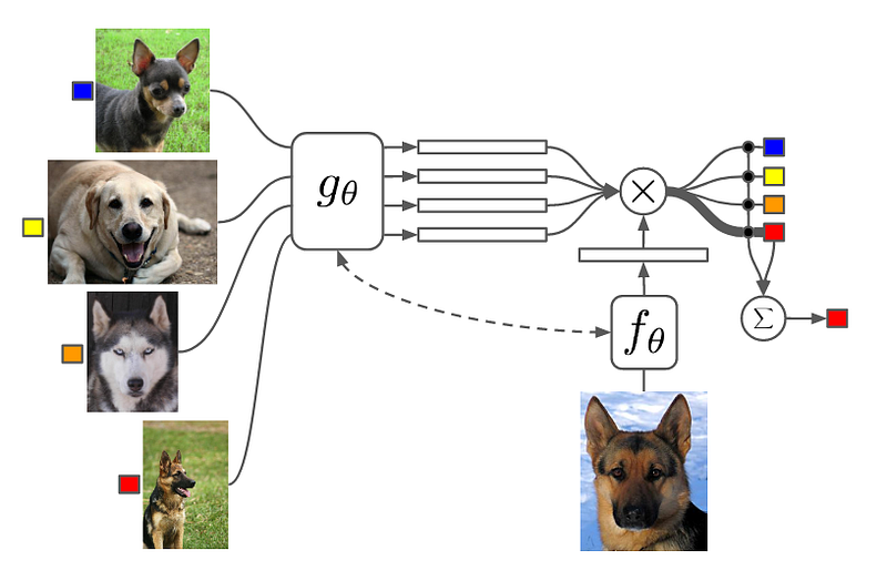
Matching Networks
combine both embedding and classification to form an end-to-end differentiable nearest neighbors classifier.
- Embed a high dimensional sample into a low dimensional space
- Perform a generalized form of nearest-neighbors classification
The meaning of this is that the prediction of the model, y^, is the weighted sum of the labels, y_i, of the support set, where the weights are a pairwise similarity function, a(x^, x_i), between the query example, x^, and a support set samples, x_i. The labels y_i in this equation are one-hot encoded label vectors.
Matching Networks are end-to-end differentiable provided the attention function a(x^, x_i) is differentiable.
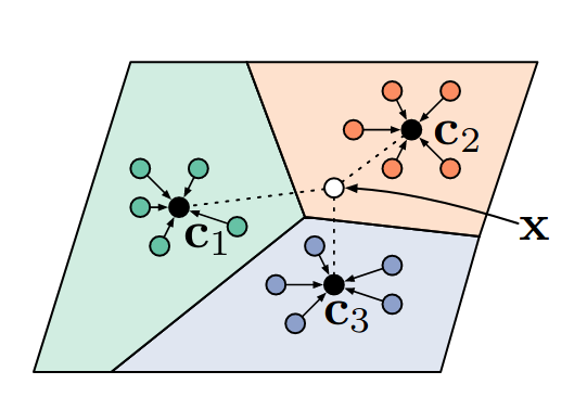
Prototypical Networks
learn class prototypes directly from a high level description of a class such as labelled attributes or a natural language description. Once you’ve done this it’s possible to classify new images as a particular class without having seen an image of that class.
- apply a compelling inductive bias in the form of class prototypes to achieve impressive few-shot performance — exceeding Matching Networks without the complication of FCE. The key assumption is made is that there exists an embedding in which samples from each class cluster around a single prototypical representation which is simply the mean of the individual samples.
- use euclidean distance over cosine distance in metric learning that also justifies the use of class means as prototypical representations. The key is to recognise that squared euclidean distance (but not cosine distance) is a member of a particular class of distance functions known as Bregman divergences.
Model-agnostic Meta-learning (MAML)
YouTube search... ...Google search
- Model-agnostic Meta-Learning: Learning to fine-tune | C. Finn, P. Abbeel, and S. Levine
- Model-Agnostic Meta-Learning for Fast Adaptation of Deep Networks (MAML)
learning a network initialization that can quickly adapt to new tasks — this is a form of meta-learning or learning-to-learn. The end result of this meta-learning is a model that can reach high performance on a new task with as little as a single step of regular gradient descent. The brilliance of this approach is that it can not only work for supervised regression and classification problems but also for reinforcement learning using any differentiable model!
MAML does not learn on batches of samples like most deep learning algorithms but batches of tasks AKA meta-batches.
- For each task in a meta-batch we first initialize a new “fast model” using the weights of the base meta-learner.
- compute the gradient and hence a parameter update from samples drawn from that task
- update the weights of the fast model i.e. perform typical mini-batch stochastic gradient descent on the weights of the fast model.
- we sample some more, unseen, samples from the same task and calculate the loss on the task of the updated weights (AKA fast model) of the meta-learner.
- update the weights of the meta-learner by taking the gradient of the sum of losses from the post-update weights . This is in fact taking the gradient of a gradient and hence is a second-order update — the MAML algorithm differentiates through the unrolled training process... optimising for the performance of the base model after a gradient step i.e. we are optimising for quick and easy gradient descent. The result of this is that the meta-learner can be trained by gradient descent on datasets as small as a single example per class without overfitting.
Siamese Networks
YouTube search... ...Google search
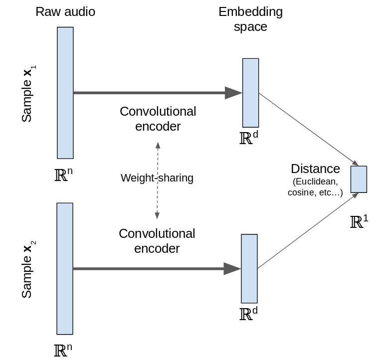
take two separate samples as inputs instead of just one. Each of these two samples is mapped from a high-dimensional input space into a low-dimensional space by an encoder network. The “siamese” nomenclature comes from the fact that the two encoder networks are “twins” as they share the same weights and learn the same function.
These two networks are then joined at the top by a layer that calculates a measure of distance (e.g. euclidean distance) between the two samples in the embedding space. The network is trained to make this distance small for similar samples and large for dissimilar samples. I leave the definition of similar and dissimilar open here but typically this is based on whether the samples are from the same class in a labelled dataset.
Hence when we train the siamese network it is learning to map samples from the input space (raw audio in this case) into a low-dimensional embedding space that is easier to work with. By including this distance layer we are trying to optimize the properties of the embedding directly instead of optimizing for classification accuracy.